
There is no doubt that the traditional picture of downward sloping demand curve and upward sloping supply curve does not apply to an asset bubble.
Downward sloping character of the demand curve is inferred from the premises of utility theory.
Someone picks a combination of goods, based on
a) Her budget constraints
b) How many units of one good she is ready to sacrifice to get an additional unit of another good (called marginal rate of substitution in utility theory).
The latter is about her tastes. She maximizes the utility for her at the point where the marginal rate of substitution equals the price ratio of two goods. The utility maximum drops to a lower level when the price of one good rises. As a result, the quantity demanded of this good diminishes. That makes the demand curve for this good downward sloping (see “Consumer choice” chapters in Microeconomics textbooks).
Yet there is no inverse relationship between price and quantity demanded in asset bubble markets. In a perfect bubble market, all participants are for the money. The higher the price at the boom phase of the market, the stronger the incentives to buy more in anticipation of even higher price. That lures more participants to enter the market. In the process, demand grows and the price increases.
At the bust phase the price falls. The participants expect the price to go down further, and the disincentives to buy emerge. As more participants withdraw from the market, demand falls and the price continues to decline, in a vicious cycle style.
Clearly, downward sloping demand curve does not hold in this case. In fact, it is upward sloping, albeit the slope, as we will see, is different for each phase of the asset bubble.
As to the supply curve, its upward sloping character holds in the situation of an asset bubble because its bottom line is the construction cost of homes (in case of housing bubble).
The graph below shows the positioning of the demand curves for two phases of an asset bubble in relation to the supply curve.
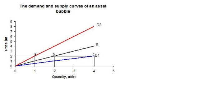
As we can see, at the upward stage of the bubble the demand curve (curve D1) is sloping upward, but the curve is positioned below the supply curve S. The slope of demand curve D1 on the graph is 0.5, and the slope of supply curve is 1 (all curves are linear, a simplification). At the price = $2M (arbitrarily picked), the difference between demand and supply is 2 units (section bc). The price is going to grow, but at the higher price, the difference is even greater. So the boom continues.
The demand curve for the deflating bubble, on the contrary, is positioned above the supply curve, which means that at any price quantity demanded is less than quantity supplied. It is about panic, after all. The slope of demand curve D2 on the graph is 2. At the price = $2M, for example, there is a surplus of units (section ab) and the price will go down. The participants will continue to withdraw from the market and the surplus persists.
If we are going to see the whole process of booming and busting, we must acknowledge that at some point of time demand curve D1 shifts to the left. Its new position is demand curve D2. It happens at the point of growing doubt, which ignites panic. Sometimes it is called Minsky Moment. Demand at Minsky Moment falls abruptly, creating a surplus.
So the demand curve exists in two forms: D1 (boom phase) and D2 (bust phase).
Suppose Minsky Moment happens when the price is $4M (this is not a real price, of course). The initial price is $1M. The slope of demand curve D1 is 0.5, the slope of demand curve D2 is 2, the slope of the supply curve is 1. All curves are linear.
To trace the trajectory of the price under these conditions we need some equations.
Let us denote:
P(t) – price at moment t, $M,
S(t) – quantity supplied at t, units,
D(t) – quantity demanded at t, units
∆P(t) – change in price at t, $M,
The equation for supply curve S is:
P(t) = S(t) (1)
The equation for demand curve D1 is:
P(t) = 0.5D(t) (2)
The equation for demand curve D2 is:
P(t) = 2D(t) (3)
Equations (1) and (2) combined represent the boom phase, equations (1) and (3), taken together, describe the bust phase of the asset bubble under the above conditions.
Price change depends on the difference between demand and supply. For illustration purposes, we assume that it is equal to the difference between demand and supply, measured in units (at this level of abstraction it does not matter how unit is defined, it might be thousands or millions of homes or condos or it might be land).
For the boom phase we get
D(t) – S(t) = P(t)/0.5 – P(t) and, substituting ∆P(t) for D(t) – S(t),
∆P(t) = P(t)/0.5 – P(t) or
∆P(t) = P(t) (4)
Given the above conditions, the price grows like this:
| P(t) $M | 1 | 2 | 4 |
| ∆P(t) $M | 1 | 2 |
Price = $4M is Minsky Moment. From this point on demand drops and the bust phase begins with shifted demand curve D2. Now we need to take equations (1) and (3).
It goes like this:
D(t) – S(t) = P(t)/2 – P(t) or
∆P(t) = P(t)/2 – P(t) or
∆P(t) = – 0.5P(t) (5)
The price at the bust phase starts at Minsky moment and falls according to (5), as the table below shows.
| P(t) $M | 4 | 2 | 1 |
| ∆P(t) $M | -2 | -1 |
Plotting all this data on the same graph, we get:
 At the starting point the price = $1M. At this price, the shortage of one unit develops and the price increases to $2M, which spawns even greater shortage of 2 units. This new shortage drives the price to $4M.
Minsky Moment has been reached. The following panic and massive withdrawal from the market crashes demand and the demand curve shifts to position D2. Resulting surplus drives the price down to $2M. Yet shortage persists at this price and the price continues to fall until it reaches $1M, the initial value. The asset bubble has deflated.
CC-BY-NC-SA
